Satellite data products potentially useful to the water node
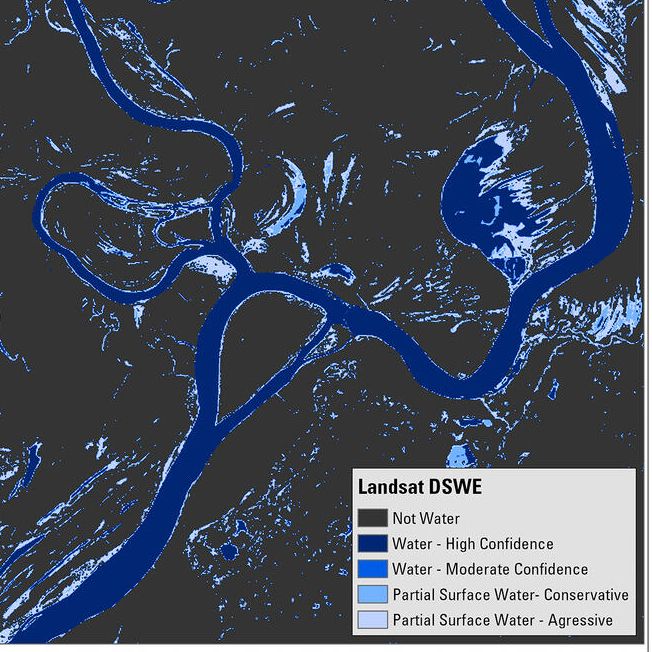
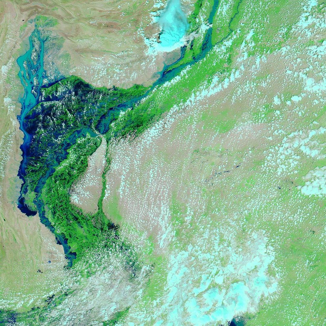
Dynamic Surface Water Extent
- Agency/Company: USGS
- Usage restrictions: public
- Resolution: 30 m
- Availability: 1982 to present. DSWE has been obtained from different landsat missions to create this dataset. For example, 1982-1992 DSWE obtained from Landsat 4.
- Sampling period: 16 days
- Similar data products: JRC Global Surface Water
The USGS’s Dynamic Surface Water Extent (DWSE) is a landsat derived satellite data source that measures the amount of surface water inundation using landsat data. It can detect the presence of surface water in any clear (cloud or shadow free) Landsat pixel. This data could potentially be useful for measuring top-width, ephemeral water, stream classification (braided, meandering, etc), monitoring river migration rates, and many other uses. Specific to NGen, Fred Ogden is excited about the possibility of obtaining top-width measurements because of the potential to relate observed changes in top width to an observed or modeled flow distribution curve. Top width measurements can also be coupled to altimetry data to produce estimates of discharge (see This presentation).
DWSE is derived from data taken from Landsat 4-5 TM, Landsat 7 ETM+, and Landsat 8 OLI/TIRS. There are two different versions of DSWE with version 1 now being effectively superseded by version 2. Sentinel data is currently being considered for inclusion in the version 2 dataset.
Current relevant uses: DSWE is currently being used to derive a database of inundation extents. This has the potential to be useful for improving FIM efforts by enabling the creation of techniques to improve FIM modeling through comparison with remotely sensed inundation extents.
More information about the dataset can be found at this page.
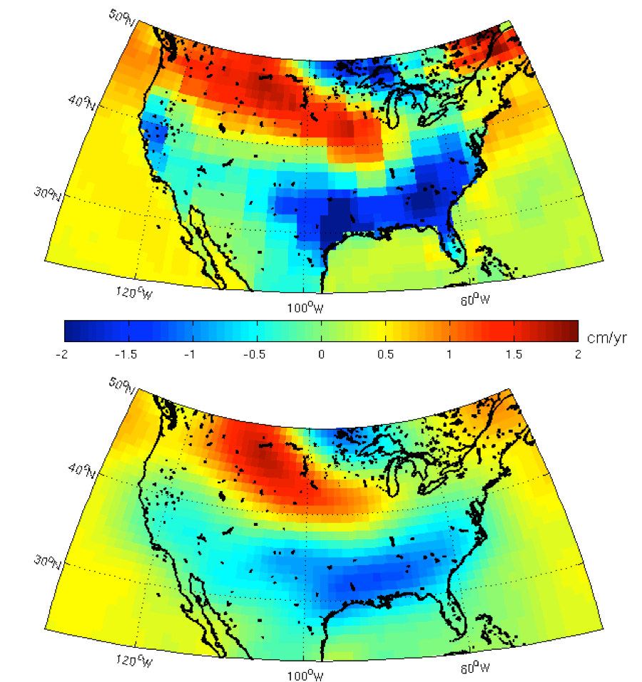
Gravity Recovery and Climate Experiment-Follow On
- Agency/Company: NASA the German Aerospace Center
- Usage restrictions: public use
- Resolution: 3 x 3 degrees latitude by longitude (300-400km)
- Availability: Data released every month.
- Sampling period: Monthly
- Similar data products: None being collected currently.
THe Gravity Recovery and Climate Experiment (GRACE) follow on mission is designed to measure fluctuations in the gravitational field of the earth. These fluctuations are primarily caused by changes in the earth’s mass distribution. GRACE is sensitive enough to pick up coarse changes in groundwater which could potentially be useful for the groundwater component of NWM in places where ground-based groundwater monitoring is limited. Using GRACE to improve estimates of groundwater is challenging due to the fact that GRACE data convolves changes in groundwater, soil moisture, snow, and surface water.
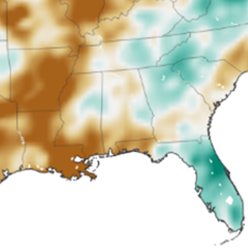
Soil Moisture Active Passive
- Agency/Company: NASA
- Usage restrictions: public use
- Resolution: 3-36 km
- Availability: Level 1-4 data products available with a maximum latency of 7 days for level 4 products and a minimum latency of 12 hrs for level 1 products.
- Sampling period: 2-3 days
- Similar data products: Soil Moisture and Ocean Salinity (SMOS) data.
The Soil Moisture Active Passive (SMAP) datasets are designed to provide rapid snapshots of soil moisture on a global scale. The moisture reading come from the top few centimeters of soil. SMAP passively measures L-band radiation to provide these estimates of soil moisture.
SMAP data has the potential to improve the runoff estimates being generated by the national water model. This is especially true in areas where the surface soil moisture reading could be coupled to groundwater depth and soil texture maps to obtain an approximate soil saturation state using a retention curve based approach. There are significant challenges associated with this approach and a brief overview of some of the challenges associated with SMAP data are given below.
To obtain a soil moisture estimate the raw L-band data must first be processed to isolate the moisture signal from other components of the L-band readings. Some factors that affect the accuracy of SMAP data are:
Vegetation cover: The microwave signals emitted by the soil can be absorbed, scattered, or reflected by vegetation. This effect becomes more pronounced with denser vegetation, making it difficult to accurately estimate soil moisture in heavily vegetated areas.
Surface roughness: The roughness of the soil surface affects the microwave radiation emitted by the soil. Rough surfaces can cause scattering of the microwave signals, which may lead to errors in soil moisture estimation.
Soil texture and composition: Different soil types have different dielectric properties, which affect the microwave radiation emitted by the soil. Obtaining good measurements of the spatial variation of soil types and texture can be challenging.
More information about the SMAP datasets can be found here
Surface Water and Ocean Topography
- Agency/Company: NASA, CNES, CSA, UK Space Agency
- Usage restrictions: public use
- Resolution: Planform resolution of 50 m for inland water and 1km for ocean. ~3cm vertical accuracy for ocean and 10cm for land.
- Availability: tentative release schedule as of April, 2023. Once data becomes available accessibility will be easier to assess.
- Sampling period: 21 days for a full cycle
- Similar data products: The altimetry data provided by Jason also gives sea surface height but does not use the Ka-band radar interferometery (KaRIn) that will be the primary instrument on SWOT. SWOT will have an altimeter that will provide surface height measurements but it will primarily be used to calibrate the KaRIn instrument.
The Surface Water and Ocean Topography (SWOT) mission is a collaborative effort between NASA and the French space agency CNES, aiming to provide high-resolution measurements of Earth’s water surface elevations for both ocean and inland water bodies.
There is great potential to use SWOT to provide remotely sensed discharge estimates for streams greater than 100 m in width. Durand et al., 2016 provides an outline of a number of different algorithms that could be used to provide remotely sensed discharge estimates using the data SWOT will make available. One of the data products that will be provided by the mission itself will be a discharge derived from SWOT data. There is also the possibility of coupling SWOT data with higher resolution measurements of water extent (for example DSWE) to improve discharge estimates.
The SWOT mission will provide a variety of datasets with initially released datasets being at processing levels 1 and 2. For the purposes of stream-flow model calibration the most immediately applicable datasets are:
- L2_HR_RiverSP
- This will provide shapefiles of river reaches with reach attributes such as slope, surface elevation, and a derived discharge estimate. The data will be provided at a finer granularity than the L2_HR_RiverAvg data described below. Data will be provided for each full-swath pass of a continent. Each swath will be ~128 km wide when measured orthogonally from the satellites track.
- L2_HR_RiverAvg
- This will provide river reach data organized by basin and averaged over all the continental passes over a given orbital cycle. L2_HR_RiverAvg will provide the min, mean, median, and max river surface elevation observed during that cycle as well as corresponding values for slope, elevation, and derived discharge.
More information about the datasets can be found here
Moderate Resolution Imaging Spectroradiometer
- Agency/Company: NASA
- Usage restrictions: public use
- Resolution: 250-1000 m depending on which band is being analyzed
- Availability: Level 1-3 data is publicly available from 3-4 different platforms. See this site for more.
- Sampling period: 1-2 day revisit period.
- Similar data products: VIIRS
MODIS refers to a sensor design that is currently on board two currently running missions. MODIS acqires data from 36 spectral bands in the wavelengths between 0.4 μm and 14.4 μm.
relevant uses for hydrological services and modelling
Flood inundation mapping
Estimating evapotranspiration
Land use maps
Links
- This tutorial gives an example of working with python to visualize global fire hotspots.
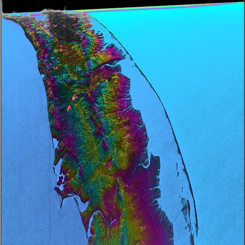
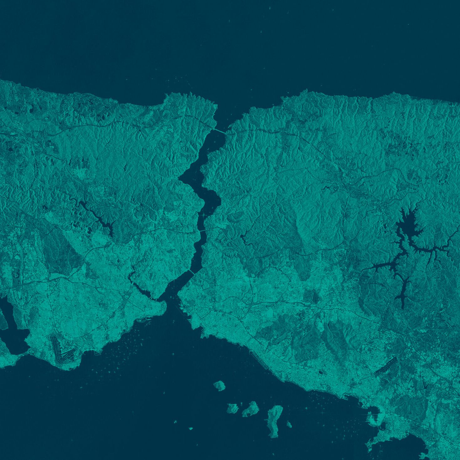
Sentinel 1
- Agency/Company: ESA
- Usage restrictions: public use
- Resolution: 5-20 m
- Availability: Level-0 through Level-2 products made available within 24 hours of observation at the Copernicus Open Access Hub. The Copernicus Sentinel Operations Dashboard provides up-to-date information regarding data availability.
- Sampling period: 6 days when using both satellites.
- Similar data products: RADARSAT, TerraSAR-X, ALOS PALSAR
(Sentinel-1A) and 2016 (Sentinel-1B), the twin satellites in the Sentinel-1 mission are equipped with Synthetic Aperture Radar (SAR) instruments that operate in the C-band, allowing them to acquire high-resolution radar imagery of Earth’s surface in all weather conditions and at any time of day. An in-depth description of available Sentinel-1 data can be found [here]
Some potential/already in-place hydrological uses of Sentinel-1 data are:
Flood inundation mapping
Sentinel-1 SAR data is already being used to improve flood inundation mapping within NOAA. SAR can penetrate clouds and function during nighttime, ensuring continuous monitoring of flood events. Its high spatial resolution (5-20 meters, depending on the acquisition mode) allows for detailed mapping of water bodies and flood extent, while its short revisit time (6 days with both satellites combined) enables near-real-time monitoring of rapidly changing hydrological conditions. For the purposes of FIM combining Sentinel-1 data with electro-optical bands acquired from other satellites holds great potential.
A database of remotely sensed flood inundation maps (some of which have been obtained from Sentinel-1) can be found here
River ice mapping
The Water Prediction Operations Division (WPOD) within the Office of Water Prediction (OWP) is also using Sentinel-1 data to map river ice. For example see this RealEarth collection.
River widths
SAR could also be used as a tool to get river extents in non-flood conditions similarly to DSWE
Soil Moisture Active Passive
- Agency/Company: NASA
- Usage restrictions: public use
- Resolution: 3-36 km
- Availability: Level 1-4 data products available with a maximum latency of 7 days for level 4 products and a minimum latency of 12 hrs for level 1 products.
- Sampling period: 2-3 days
- Similar data products: Soil Moisture and Ocean Salinity (SMOS) data.
The Soil Moisture Active Passive (SMAP) datasets are designed to provide rapid snapshots of soil moisture on a global scale. The moisture reading come from the top few centimeters of soil. SMAP passively measures L-band radiation to provide these estimates of soil moisture.
SMAP data has the potential to improve the runoff estimates being generated by the national water model. This is especially true in areas where the surface soil moisture reading could be coupled to groundwater depth and soil texture maps to obtain an approximate soil saturation state using a retention curve based approach. There are significant challenges associated with this approach and a brief overview of some of the challenges associated with SMAP data are given below.
To obtain a soil moisture estimate the raw L-band data must first be processed to isolate the moisture signal from other components of the L-band readings. Some factors that affect the accuracy of SMAP data are:
Vegetation cover: The microwave signals emitted by the soil can be absorbed, scattered, or reflected by vegetation. This effect becomes more pronounced with denser vegetation, making it difficult to accurately estimate soil moisture in heavily vegetated areas.
Surface roughness: The roughness of the soil surface affects the microwave radiation emitted by the soil. Rough surfaces can cause scattering of the microwave signals, which may lead to errors in soil moisture estimation.
Soil texture and composition: Different soil types have different dielectric properties, which affect the microwave radiation emitted by the soil. Obtaining good measurements of the spatial variation of soil types and texture can be challenging.
More information about the SMAP datasets can be found here
Design of water node website
Implementing a static STAC catalog
Static STAC catalogs are STAC collections that are stored as files on a server or a cloud bucket. For the water node it was decided that
Getting data into S3 bucket
Will this change be reflected?
Computing an extent using a HAND input
Script to compute extents “inundate_mosaic_wrapper.py
Inputs The FIM4 outputs are organized by HUC8. Inside of each HUC8 folder
the files needed to run inundation.py are:
hydrotable.csv. This file contains HAND-derived variables describing the channel/overbank geometry and corresponding synthetic rating curve attributes for each flowline.
rem_zeroed_masked.tif. This file is the Relative elevation model raster with pixel values representing the height above nearest drainage (Note: negative values removed and masked to the HUC boundary)
gw_catchments_reaches_filtered_addedAttributes.tif. Raster with pixel values representing the catchment HydroID value
gwcatchments_reaches_filtered_addedAttributes_crosswalked.gpkg. Multipolygon layer containing a catchment polygon for each HydroID stream segment with crosswalked NWM feature_id attribute.
forecast file. This has the forecast discharges. This can be a csv where the columns headers correspond to: feature_id (NWM feature id) and discharge value.
Importing HAND extents into postGIS
Want the extents to be in the wgs 1984 projection since that is what everything else ended up being in.
Hierarchy of Orginazational Topologies
Things get done at a point. Keep coming back to what you are doing.
Points get provisionally strung along a line. So respect the line next. Use a calendar to situate tasks in time. This allows you to not become overwhelmed. As much as possible when a task comes in try to assign a date and time to work on that thing. If it doesn’t get done and still needs to then assign it to a new time or break down the task and assign these smaller tasks to new times. If a task keeps getting pushed back drop it or create the conditions that make it absolutely necessary that it happen. Only schedule from hour after waking to end of workday most days and try to keep space 3-5 days out in calendar (like 30-50) empty so that things can be moved around.
Keep one big text file representing a daily schedule and a log of what happens as you try to follow that schedule is useful. So the day’s schedule/tasks get transferred from calendar to your logfile. Throughout the day take notes on what you are doing, feeling, and thinking. It doesn’t have to be structured just get it out. This is the space to think out loud and do provisional planning. If you write enough in the log then due to the nature of language thoughts start to take on a treelike shape. Occasionally new documents or additions to long-form documents describing a project or different aspects of your projects will emerge naturally.
Tend to the trees/documents in separate files that you work on in public as much as possible. Every Friday push updates to these trees/long form documents to a public, pseudonymous weblog. Carve out 90 minutes or so once a week to go back over the previous weeks log and look for stuff that hasn’t yet been integrated into a document. The idea is to go from scrap to something being shared as quickly as possible. As you iterate on these project descriptions, communicate with other people, and review the previous days activities tasks/next steps will suggest themselves and you can add them onto the schedule.
A bunch of trees/documents can be linked into a graph and in a large enough document a graph structure from resonant or explicit links will start to emerge.
While each topology is useful there is also a sense in which each is more phantasmic than the other. Dreams on top of dreams until the dreams create the net within which reality is co-created. From the perspective of a limited being giving priority to what is happening right now and situating yourself in time makes the most sense since it allows you to work with your most finite resource (time) not against it. Then viewing descriptions (the trees and graphs) as potential models/contexts that are of secondary importance. The contexts are there to help guide the action. You aren’t living to create a theory you are creating
Related posts: Anchor yourself in time
Generating ground based calisthenic workouts
- Squat
- lunge
- side squat
- crab
- standing
- on stomach
- on back
- beast
- L-sit
today’s numbers: 9, 1, 3
generate random sequences of 3 from these movements. Start with 27 reps and add one a day until get to 54. If you miss a day fall back to 27.
So the transitions generated by the juxtapositions are just as important as the moves themselves. Striving to do the transitions gracefully as you repeat the set. Don’t have to codify the transitions.
When a unilateral movement comes up use your creativity to find a way to do both sides in the context of the sequence. For example if you go bilateral to unilateral you can go unilateral then back to bilateral. If the sequence starts with unilateral then goes to another unilateral then experiment as you repeat the flow.
Try not to hit full standing in transitions that don’t have standing. The transition will be more challenging and useful if you don’t “reset” by adding intermediate poses. The exception to this is transitioning into and out of lunges.
Disallow repetitions for sake of simplicity.
So incorporate variety in a routine way while using the repetition inside the workout to cultivate devotion. Each workout is a call to both creation and devotion.